Load Balancing Algorithms: How Traffic Is Distributed
Series: System Design · Scalability & Infrastructure — Pillar 6 of 8
Systems Design
| # | Post | What it covers |
|---|---|---|
| 00 | Scalability & Infrastructure: The Layer Between Your Code and the Internet | Nine concepts covering load balancing, rate limiting, proxies, compression, and probabilistic data structures that keep large systems fast and reliable. |
| 01 | Client-Server Architecture: The Model Everything Else Builds On | Client-server is the foundational model for distributed systems. Learn what clients and servers know, where state lives, and how the model scales. |
| 02 | Load Balancing: Distributing Traffic Across Servers | Load balancers distribute traffic across servers for scale and availability. Learn how they work, what types exist, and what they require of backend servers. |
| 03 | Load Balancing Algorithms: How Traffic Is Distributed ← you are here | Round robin, least connections, IP hash, weighted — each algorithm makes different tradeoffs. Learn how to choose the right one for your workload. |
| 04 | Rate Limiting: Protecting Services from Overload | Rate limiting protects services from overload and abuse. Learn how token bucket, leaky bucket, and sliding window algorithms work and when to use each. |
| 05 | Proxy vs Reverse Proxy: Which Way Does It Face? | Forward proxies protect clients; reverse proxies protect servers. Learn how each works, what Nginx and Cloudflare do, and when you need which. |
| 06 | Data Compression: Smaller, Faster, Cheaper | Compression reduces bandwidth and storage costs. Learn how Gzip, Brotli, LZ4, and zstd work, where to apply them, and the CPU tradeoffs involved. |
| 07 | Checksums: Detecting Corruption Before It Becomes a Catastrophe | Checksums detect silent data corruption in transit and storage. Learn how CRC32, MD5, and SHA-256 work and where to apply them in distributed systems. |
| 08 | Bloom Filters: Answering "Have I Seen This?" Without Storing Everything | A Bloom filter answers "have I seen this?" in constant memory. Learn how they work, why false positives are acceptable, and where they're used in production. |
| 09 | HyperLogLog: Counting Distinct Items Without Storing Them | HyperLogLog counts distinct values in ~1.5 KB of memory with <2% error. Learn how it works and why Redis, BigQuery, and Postgres use it. |
| 10 | Scalability & Infrastructure: Wrap-Up | A recap of all 9 scalability concepts: load balancing, rate limiting, proxies, compression, checksums, Bloom filters, and HyperLogLog. How they fit together. |
Load Balancing Algorithms: How Traffic Is Distributed
The problem
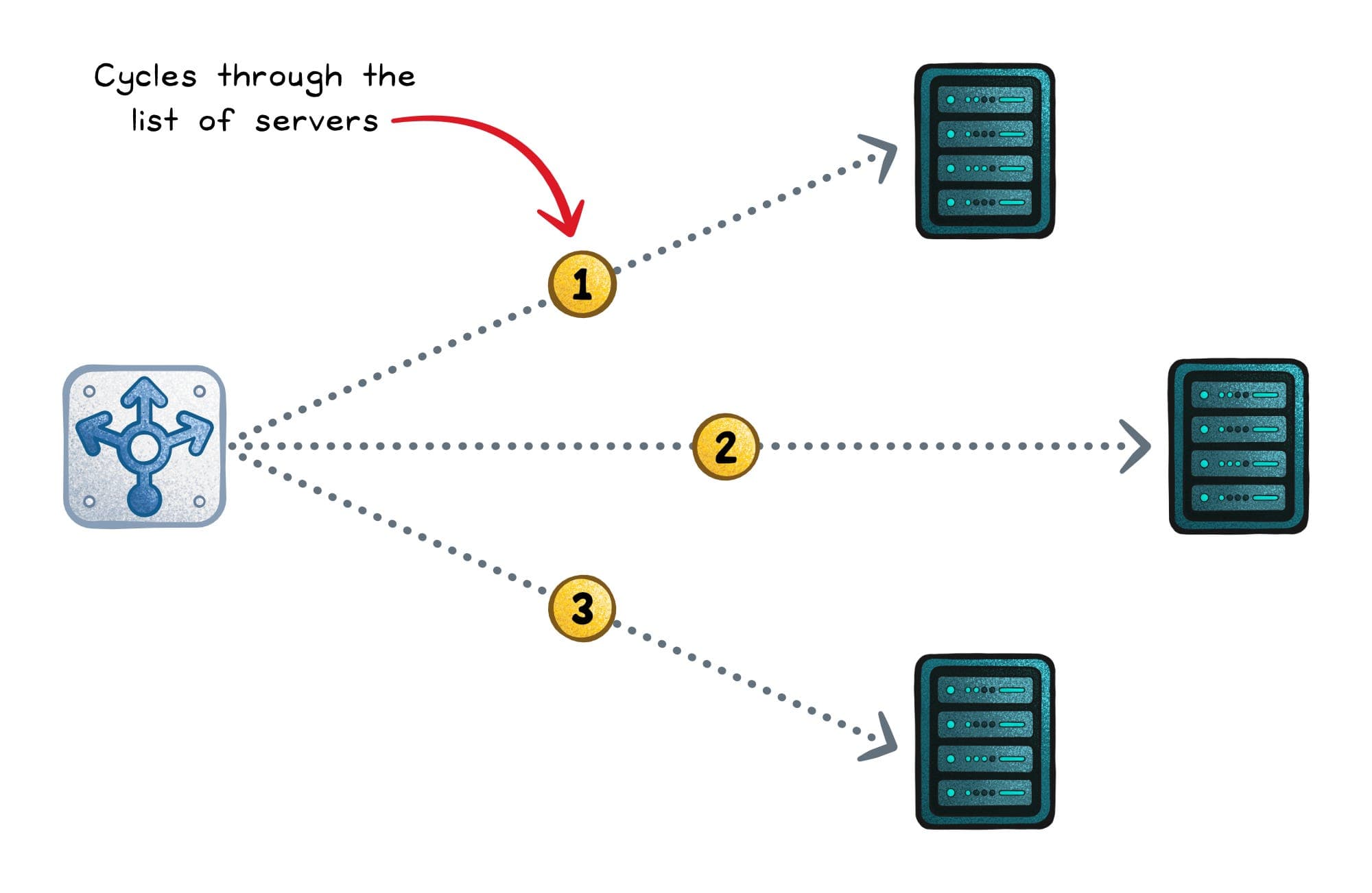
A load balancer must answer one question on every incoming request: which backend server should handle this?
The simplest answer — "the next server in the list, cycling forever" — works fine when every request takes the same amount of time and every server has the same capacity. In practice, neither is true. Some requests take a millisecond; others take two seconds. Some servers have 32 cores; others have 8. Some clients need all their requests to go to the same server; others don't care.
The wrong algorithm under the wrong workload creates hotspots — one server overwhelmed while others are idle — or breaks features that require session consistency. The right algorithm is the one that matches your request distribution, server topology, and stickiness requirements.
The core idea
A load balancing algorithm is the decision procedure the load balancer uses to select a backend server for each request. Each algorithm optimises for a different property: fairness, latency, stickiness, or ability to handle heterogeneous server pools.
The analogy: assigning tasks in an office
Imagine a team lead distributing incoming customer emails to a support team.
- Round robin: assign emails 1, 2, 3... cycling through each team member in order. Everyone gets equal volume — but if email 7 takes four hours while others take ten minutes, one person is buried while others have idle time.
- Least connections: assign the next email to whoever has the fewest active emails in their queue. More work-aware — naturally routes to whoever is done with previous work first.
- IP hash: always route emails from the same customer to the same team member. Useful when the team member builds context about that customer.
- Weighted: a senior agent gets 3x more emails than a junior one, reflecting different capacity.
Each rule serves a different team structure and email type.
The main algorithms
Round Robin
Cycle through backend servers in sequence: request 1 → Server A, request 2 → Server B, request 3 → Server C, request 4 → Server A, ...
Servers: [A, B, C]
Requests: 1→A, 2→B, 3→C, 4→A, 5→B, 6→C ...
Strengths: Simple. Zero state beyond a counter. Even distribution assuming uniform request cost and equal server capacity.
Weaknesses: Ignores request duration. If Server A gets a mix of 1ms and 10-second requests while Server B gets only 1ms requests, Server A accumulates a backlog. Ignores server capacity — a 4-core server and a 32-core server get the same number of requests.
Best for: Homogeneous servers, roughly uniform request cost, stateless requests. The most common default.
Weighted Round Robin
Round robin with a multiplier. Server A (weight 3) gets three requests for every one request to Server B (weight 1).
Servers: [A(weight=3), B(weight=1)]
Requests: 1→A, 2→A, 3→A, 4→B, 5→A, 6→A, 7→A, 8→B ...
Strengths: Matches traffic distribution to server capacity. Allows heterogeneous server pools (large and small instances sharing load proportionally).
Weaknesses: Still ignores actual server load — a weight-3 server that happens to be processing three long-running requests gets more traffic anyway.
Best for: Mixed instance sizes (some servers larger than others), gradual rollout (new servers start with low weight, increase as confidence grows).
Least Connections
Route each request to the server with the fewest currently active connections.
Server A: 12 active connections
Server B: 4 active connections  ← next request goes here
Server C: 9 active connections
Strengths: Adapts to variable request duration. Long-running requests (database migrations, file uploads, slow analytics queries) accumulate on whichever server got them; new short-lived requests route to servers that are more available. Self-balancing under heterogeneous load.
Weaknesses: Requires the load balancer to track active connection counts per backend — slightly more overhead than round robin. Can behave unexpectedly during connection spikes if many connections open simultaneously before any close.
Best for: Workloads with variable request duration (mix of fast and slow requests). The most robust general-purpose algorithm when request cost is non-uniform.
Least Response Time
Route to the server with the lowest average response time (often combined with least connections: lowest connections × average_response_time).
Server A: avg 45ms response, 10 connections
Server B: avg 12ms response, 8 connections  ← routes here
Server C: avg 80ms response, 3 connections
Strengths: Actively accounts for server health and performance, not just connection count. Routes away from degraded servers automatically.
Weaknesses: Response time averaging requires more state (rolling average per backend). Can oscillate — a server just finished a slow request has a momentarily poor average, misses new requests, its average improves, gets flooded again.
Best for: Workloads where response time varies based on server health or load, and you want the load balancer to actively route to healthier servers.
IP Hash (Source IP Affinity)
Hash the client's IP address to determine the backend server. The same client IP always routes to the same server.
Client 203.0.113.42 → hash → Server B (always)
Client 198.51.100.7 → hash → Server A (always)
Strengths: Provides sticky sessions without a cookie or shared session store. Useful for stateful backends or when the backend builds per-client state (connection pooling, session context).
Weaknesses: Load distribution is only as even as IP distribution — if many clients share an IP (corporate NAT, a large mobile carrier), one server gets all of them. Doesn't account for server load. Server failure breaks stickiness for clients mapped to that server.
Best for: Stateful backends where you need session affinity without modifying the application. Less preferable to cookie-based stickiness, which is more reliable.
Consistent Hashing
Hash the request key (URL path, user ID, session ID) to a position on a ring. Route to the nearest server on the ring. Adding or removing a server only remaps ~1/N of keys.
Ring:
  url:x7Kp2 → position 35% → Server B
  url:aB3cD → position 72% → Server C
Strengths: Minimises remapping on topology changes. Natural fit for cache-aware load balancing — if backend servers maintain local caches, routing the same request to the same server maximises cache hit ratio.
Weaknesses: More complex to implement. Requires a consistent hashing client library. The server selected may not be the least loaded.
Best for: Cache servers, stateful session routing, systems where cache locality matters (always hit the same server for the same URL so in-memory cache is warm).
Random
Select a backend at random for each request.
Strengths: Trivially simple. No state. Statistically produces even distribution over large numbers of requests.
Weaknesses: No adaptation to server load, health, or latency. High variance for small request volumes.
Best for: Rarely. Round robin almost always dominates random. Useful in specific probabilistic load spreading scenarios.
Choosing an algorithm
| Workload | Recommended algorithm |
|---|---|
| Uniform requests, equal servers | Round robin |
| Mixed instance sizes | Weighted round robin |
| Variable request duration | Least connections |
| Performance-sensitive, heterogeneous | Least response time |
| Stateful backend (legacy) | IP hash or cookie-based sticky |
| Cache-aware routing | Consistent hashing |
| Static content, CDN layer | Consistent hashing |
For the URL shortener:
- Redirect endpoint: round robin (requests are fast and uniform; stateless)
- API endpoints (link CRUD, analytics): least connections (variable duration — some analytics queries are slower)
- The cache layer's client-side routing: consistent hashing (all requests for a given link key hit the same Redis shard)
Tradeoffs
Simplicity vs adaptation. Round robin is simplest and works well under uniform conditions. Least connections adapts but requires tracking state. Least response time adapts better but requires more complex state and can oscillate.
Stickiness vs flexibility. IP hash and consistent hashing provide affinity but sacrifice load-based routing. A server that happens to be slow still receives its full share.
Health integration. All algorithms should be combined with health checks — an algorithm that doesn't remove unhealthy servers from consideration routes into failures regardless of how sophisticated the selection logic is.
The one thing to remember
The load balancing algorithm determines not just distribution but adaptation. Round robin assumes all requests and all servers are equal — when they're not, it creates hotspots. Least connections adapts to variable request duration without knowing anything about what the requests are doing. Match the algorithm to the nature of your workload: if your requests are fast and uniform, round robin is sufficient; if they vary in duration or cost, least connections is more robust.
← Previous: Load Balancing — when a single server can't handle all the clients, a load balancer distributes them across a pool — here's how that works and what it requires of the servers behind it.
→ Next: Rate Limiting — even a perfect load balancer needs a mechanism to protect services from clients that send too many requests.