Erasure Coding: Fault Tolerance Without Full Replication
Series: System Design · Distributed Systems — Pillar 8 of 8
Systems Design
| # | Post | What it covers |
|---|---|---|
| 00 | Distributed Systems: What Happens When Machines Disagree | Twenty concepts covering network partitions, consensus, clocks, distributed transactions, CDC, erasure coding, and observability. The final pillar. |
| 01 | Network Partitions: The Failure Mode You Can't Design Away | Network partitions are inevitable. Learn what happens when nodes can't communicate, how systems choose between availability and consistency, and what that means in practice. |
| 02 | Split-Brain: When Two Nodes Both Think They're the Leader | Split-brain occurs when two nodes both believe they're the primary. Learn how it happens, why it causes data corruption, and how STONITH and fencing prevent it. |
| 03 | Heartbeats: How Nodes Know Their Peers Are Alive | Heartbeats let nodes detect peer failures. Learn how timeouts, phi accrual failure detectors, and the tradeoff between false positives and detection speed work. |
| 04 | Leader Election: Agreeing on Who's in Charge | Leader election coordinates which node acts as primary. Learn the bully algorithm, Raft-based election, and why exactly-one-leader guarantees are hard to achieve. |
| 05 | Consensus Algorithms: Agreeing on a Value Across Failures | Consensus lets distributed nodes agree on a value despite failures. Learn what FLP impossibility means, what Paxos and Raft provide, and where consensus is used. |
| 06 | Quorum: How Many Nodes Must Agree? | Quorum determines how many nodes must agree for an operation to succeed. Learn how R + W > N ensures consistency in distributed databases like Cassandra and DynamoDB. |
| 07 | Paxos: The Algorithm That Started It All | Paxos is the foundational distributed consensus algorithm. Learn how its two phases work, why it's hard to implement, and what systems use it in production. |
| 08 | Raft: Consensus Made Understandable | Raft makes distributed consensus understandable. Learn how leader election, log replication, and safety work in the algorithm that powers etcd, CockroachDB, and TiKV. |
| 09 | Gossip Protocol: Decentralised Cluster Communication | Gossip protocols propagate information across a cluster without a central coordinator. Learn how epidemic spreading works and where it's used in production. |
| 10 | Logical Clocks: When Physical Time Isn't Enough | Physical clocks drift and can't establish event order in distributed systems. Logical clocks track causality instead. Learn why this matters and how it works. |
| 11 | Lamport Timestamps: Ordering Events Without a Global Clock | Lamport timestamps assign logical counters to events to establish causal order in distributed systems. Learn how they work and what they can and can't tell you. |
| 12 | Vector Clocks: Knowing When Events Are Truly Concurrent | Vector clocks detect causality and concurrency in distributed systems. Learn how they work, how Dynamo uses them for conflict detection, and their limitations. |
| 13 | Distributed Transactions: When One Machine Isn't Enough | Distributed transactions are hard. Learn why cross-service atomicity is expensive, when to use it, and when eventual consistency is the right alternative. |
| 14 | Two-Phase Commit: Coordinating a Distributed Decision | 2PC ensures distributed atomicity through prepare and commit phases. Learn how it works, the coordinator failure problem, and why it's rarely used in modern systems. |
| 15 | Three-Phase Commit: Solving 2PC's Blocking Problem | 3PC adds a pre-commit phase to eliminate 2PC's blocking problem. Learn how it works, what assumptions it requires, and why it's rarely used in production. |
| 16 | Delivery Semantics: What Does "Delivered" Actually Mean? | Message delivery guarantees define system reliability. Learn what at-most-once, at-least-once, and exactly-once mean, what they cost, and when each is appropriate. |
| 17 | Change Data Capture: Streaming Your Database in Real Time | CDC streams database changes in real time by reading the write-ahead log. Learn how Debezium works, what CDC enables, and when to use it. |
| 18 | Erasure Coding: Fault Tolerance Without Full Replication ← you are here | Erasure coding stores data across nodes using math, not full replication. Learn how Reed-Solomon works, how S3 uses it, and when it beats 3x replication. |
| 19 | Merkle Trees: Efficiently Finding What's Different | Merkle trees efficiently detect which parts of a large dataset differ between nodes. Learn how Bitcoin, Cassandra, and Git use them for verification and anti-entropy. |
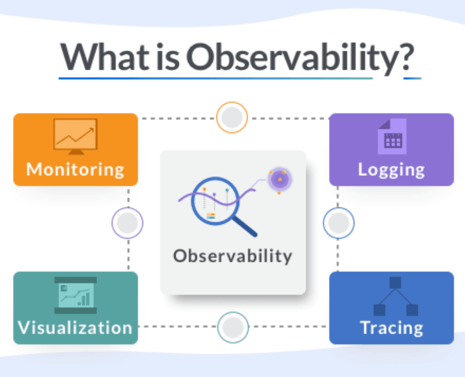
| 20 | Observability: Understanding Your System at Runtime | Logs, metrics, and distributed traces are how you understand a system at runtime. Learn what each pillar provides, the tools involved, and how they work together. |
| 21 | Distributed Systems: Wrap-Up | A recap of all 20 distributed systems concepts and the complete URL shortener architecture spanning all 8 pillars. The final post in the series. |
Erasure Coding: Fault Tolerance Without Full Replication
The problem
Amazon S3 stores every object with eleven nines (99.999999999%) durability — the probability of losing an object is essentially zero. If S3 achieved this through 3× replication (three full copies of every object), storing 1 PB of data would require 3 PB of raw storage. At S3's scale (hundreds of exabytes), this is an enormous storage overhead.
Is there a way to achieve the same durability guarantee with less storage overhead?
Yes: erasure coding.
The core idea
Erasure coding divides data into k data chunks, encodes them into n total chunks (n > k) using a mathematical transformation, and distributes the n chunks across n nodes. Any k of the n chunks are sufficient to reconstruct the original data. The system can tolerate losing up to n − k chunks (nodes) without data loss.
The overhead: n/k instead of a full replication factor. A common configuration is 10+4 (k=10, n=14): the original data is encoded into 14 chunks; any 10 are sufficient for recovery; 4 nodes can fail without data loss. Storage overhead: 14/10 = 1.4× — versus 3× replication for equivalent fault tolerance.
The analogy: a torn photograph reconstructed from fragments
A photograph is cut into 14 pieces and distributed to 14 people. The rule: any 10 of the 14 pieces are sufficient to reconstruct the complete photograph. Even if 4 people lose their pieces, the photograph can still be recovered from the remaining 10.
The encoding adds some redundancy (14 pieces instead of 10 direct copies), but far less redundancy than keeping 3 complete photographs.
How erasure coding works (interactive diagram)
Reed-Solomon codes
The most common erasure coding scheme. The original data is treated as a polynomial; the k data chunks are the polynomial's coefficients. The n total chunks are evaluations of the polynomial at n distinct points. Any k evaluations are sufficient to recover the original polynomial (and thus the data) through polynomial interpolation.
Original data: 10 chunks of 100 MB each = 1 GB

Encoding (10+4 Reed-Solomon):
  Compute 4 additional "parity" chunks using polynomial math
  Result: 14 chunks × 100 MB = 1.4 GB stored (1.4× overhead)

  Any 10 of 14 chunks reconstruct the original
  System tolerates loss of any 4 chunks (nodes)

vs 3× replication:
  3 complete copies × 1 GB = 3 GB stored (3× overhead)
  Tolerates loss of any 2 copies
The reconstruction process (interactive diagram)
If a node fails and its chunk is lost, the system must reconstruct it:
Read any k surviving chunks
Apply the inverse Reed-Solomon transform (polynomial interpolation)
Recover the original data
Re-encode the missing chunk
Write the recovered chunk to a replacement node
This is more computationally expensive than simply copying a replica — reconstruction requires reading k chunks and computing the inverse transform. For large objects, reconstruction is I/O and CPU intensive.
Where erasure coding is used
Amazon S3: uses erasure coding internally (specific scheme not disclosed). Objects are split across multiple storage nodes; the system can recover from multiple simultaneous node failures.
HDFS (Hadoop): HDFS 3.x supports erasure coding via EC policies. Common configuration: 6+3 (6 data blocks, 3 parity blocks). For cold data that's rarely accessed, erasure coding reduces storage from 3× to 1.5× while maintaining the same fault tolerance.
Ceph: supports erasure-coded pools alongside replicated pools. Cold data goes to EC pools for storage efficiency.
Meta's Tectonic: Meta's internal distributed filesystem uses erasure coding for the vast majority of cold data storage.
RAID 5/6 (local disks): the familiar RAID scheme is erasure coding: RAID 5 is k+1 (one parity disk), RAID 6 is k+2 (two parity disks).
Tradeoffs
Storage efficiency vs recovery cost. Erasure coding is more storage-efficient than replication. The cost: recovery requires reading k chunks (more I/O than copying one replica) and computing the inverse transform (more CPU). For hot data accessed frequently, the reconstruction cost makes erasure coding impractical.
Write overhead. Writing a new object requires computing all n chunks (encoding), not just writing k copies. Encoding is fast (Reed-Solomon is a well-optimised operation), but it's more work than a simple replicate-and-write.
Latency. Reading an erasure-coded object requires reading from k nodes simultaneously. Network round-trips to k nodes add latency compared to reading from the nearest replica.
Best for cold/archive data. Erasure coding's efficiency advantage is most valuable for large, infrequently accessed datasets (backups, logs, cold storage). For frequently accessed hot data, replication's simpler read path (read from nearest replica, no reconstruction) usually wins.
The one thing to remember
Erasure coding achieves fault tolerance with less storage overhead than replication by splitting data into k data chunks and n−k parity chunks, such that any k of the n total chunks reconstruct the original. A 10+4 configuration tolerates 4 node failures with only 40% storage overhead — versus 200% overhead for 3× replication. The cost is more complex reads and writes, and expensive reconstruction when chunks are lost. Erasure coding is the right choice for large, cold datasets where storage cost matters more than read performance.
← Previous: Change Data Capture — streaming database changes in real time by reading the write-ahead log.
→ Next: Merkle Trees — efficiently comparing large datasets across distributed nodes to find which parts have diverged.