Series: System Design · Architecture Patterns — Pillar 7 of 8

Systems Design

#	Post	What it covers
00	Architecture Patterns: How Systems Are Structured	Twenty patterns covering monoliths, microservices, events, resilience, deployment, and data processing. How to structure systems that survive growth.
01	Monolithic Architecture: The Default That Gets Abandoned Too Early	Monoliths are fast to build and easy to operate. Learn when they're the right choice, when they break down, and how to know the difference.
02	Microservices: The Architecture You Earn, Not Choose	Microservices enable independent scaling and team autonomy — but at significant cost. Learn what you actually get, what you pay, and when it's worth it.
03	Serverless: Pay for What You Use, Not What You Provision	Serverless scales to zero and charges per invocation. Learn where it shines, where it fails, and how to design around cold starts and vendor lock-in.
04	Event-Driven Architecture: Decoupling Through Events	Event-driven systems communicate via events rather than direct calls. Learn how producers, consumers, and event brokers work — and the consistency tradeoffs involved.
05	Message Queues: Decoupling Produce from Consume	Message queues decouple producers and consumers, enable load levelling, and provide durability. Learn how they work and when to use Kafka vs SQS vs RabbitMQ.
06	Pub/Sub: Broadcasting Events to Multiple Consumers	Pub/sub decouples publishers from subscribers through topics. Learn how it differs from message queues and when to use Kafka, SNS, or Google Pub/Sub.
07	CQRS: When Reads and Writes Need Different Models	CQRS separates writes from reads so each can be optimised independently. Learn how it works, when it's worth the complexity, and when it isn't.
08	Event Sourcing: The Ledger, Not the Balance	Event sourcing stores state as a sequence of events. Learn how it works, what you get (audit log, time travel), and what it costs (complexity, schema evolution).
09	The Saga Pattern: Distributed Transactions Without Locks	The Saga pattern manages distributed transactions across services using compensating transactions. Learn choreography vs orchestration and when to use each.
10	The Outbox Pattern: Atomic Writes and Event Publishing	The Outbox pattern solves the dual-write problem — publishing an event and writing to a database atomically. Learn how it works using CDC or polling.
11	The Circuit Breaker: Stopping Cascading Failures	Circuit breakers prevent cascading failures by fast-failing calls to unhealthy dependencies. Learn the three states, how to configure them, and where to apply them.
12	The Bulkhead Pattern: Containing Failures Through Resource Isolation	Bulkheads isolate thread pools and connections per dependency so one failure can't exhaust resources needed by others. Learn how to apply them in practice.
13	The Sidecar Pattern: Cross-Cutting Concerns Without Code Changes	The sidecar pattern deploys a helper process alongside each service for logging, metrics, TLS, and service discovery — without modifying the service itself.
14	Service Mesh: A Programmable Network for Microservices	A service mesh handles service-to-service traffic, mTLS, circuit breaking, and observability via a fleet of sidecar proxies. Learn how it works and when to use it.
15	Service Discovery: Finding Services in a Dynamic Environment	Service discovery lets services find each other in dynamic environments. Learn client-side vs server-side discovery, health checks, and DNS vs registry approaches.
16	The Strangler Fig: Replacing a Legacy System Without Burning It Down	The Strangler Fig replaces a legacy system incrementally by routing specific functionality to new implementations while the old system keeps running.
17	Backend for Frontend: One API Per Client Type	BFF creates dedicated API backends per client type. Learn why one general API struggles to serve mobile and web well, and how BFF solves it.
18	ETL Pipelines: Moving Data from Operations to Analytics ← you are here	ETL moves data from operational systems into analytical stores. Learn how pipelines work, what ELT is, and how to design reliable data movement at scale.
19	Batch vs Stream Processing: How Fresh Do Your Answers Need to Be?	Batch processes accumulate data then processes in bulk; streaming processes each event as it arrives. Learn the tradeoffs and when each is right.
20	MapReduce: Processing Petabytes in Parallel	MapReduce processes massive datasets in parallel by splitting work into map and reduce phases. Learn how it works and why Spark has largely replaced it.
21	Architecture Patterns: Wrap-Up	A recap of all 20 architecture patterns across decomposition, async communication, data patterns, resilience, and data processing. How they connect.

---

ETL Pipelines: Moving Data from Operations to Analytics

The problem

Your URL shortener's PostgreSQL database handles link management and user accounts. The analytics team wants to answer questions like: "Which industries create the most links? What percentage of links created in January were still active in June? Which pricing tier has the highest link-per-user density?"

These are multi-table, multi-period aggregate queries that would be catastrophic to run against the production operational database. They'd lock tables, consume all query capacity, and potentially degrade redirect performance — the core product function — for users.

Even if the queries were fast, the production database schema is optimised for transactional operations: normalised tables, foreign keys, row-level locks. An analytical query that needs to join five tables and aggregate a year of data is a completely different access pattern.

You need to get the data into a separate system — one designed for analytics, not transactions — and keep it up to date.

---

The core idea

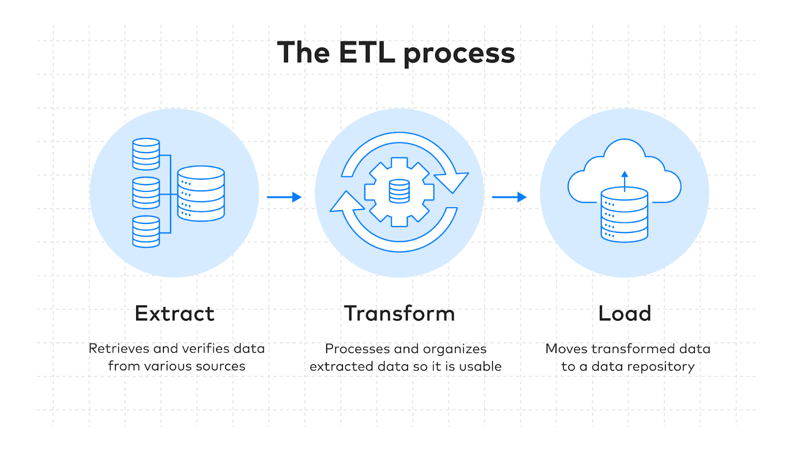
ETL (Extract, Transform, Load) is the process of moving data from operational sources into an analytical destination:

• Extract: pull data from the operational source (PostgreSQL, Cassandra, Kafka, third-party APIs)

• Transform: reshape, clean, enrich, and aggregate the data into an analytical schema

• Load: write the transformed data to the destination (data warehouse, data lake)

The separation between source and destination allows each to be optimised for its purpose: the operational database for fast transactional reads and writes; the analytical store for fast aggregation queries over large datasets.

---

The analogy: a daily news summary

A newspaper reporter (operational database) records everything that happens — raw facts, in real time, in a format that's useful for reporting. A news summary writer (ETL pipeline) takes the day's raw reports, extracts the relevant stories, rewrites them into a coherent narrative format (transform), and publishes the summary edition (load). The summary is a different format from the raw reports — it's optimised for reading and comprehension, not for recording new facts.

---

How ETL works

Extract

Pull data from one or more sources. Three strategies:

Full extract: copy the entire source table on every run. Simple but expensive for large tables. Appropriate for small, slow-changing reference data.

Incremental extract: copy only rows that changed since the last run, using a updated_at timestamp or a change sequence number.

-- Incremental: only links updated since last ETL run
SELECT * FROM links
WHERE updated_at > :last_run_timestamp
   OR created_at > :last_run_timestamp

CDC (Change Data Capture): stream changes from the source database's write-ahead log using a tool like Debezium. Near-real-time, minimal source load, but requires WAL access.

Transform

Convert the extracted data into the analytical schema:

• Normalise: standardise values (country codes, device types, URL formats)

• Enrich: join with reference data (look up company size from domain, timezone from IP)

• Aggregate: pre-compute rollups (daily click counts per link per country)

• Reshape: pivot from row-based to column-based, flatten nested structures, split combined fields

• Clean: handle nulls, remove invalid records, deduplicate

def transform_click_events(raw_clicks):
    return [
        {
            "link_id": click["link_id"],
            "date": parse_date(click["clicked_at"]),
            "country_code": normalise_country(click["geo_ip"]),
            "device_type": classify_device(click["user_agent"]),
            "is_unique": click["is_unique_visitor"]
        }
        for click in raw_clicks
        if click["link_id"] is not None  # filter invalid records
    ]

Load

Write transformed data to the destination. Two patterns:

Replace: truncate the destination table and write the full transformed dataset. Simple but risky for large tables (downtime during swap) and inefficient (rewriting unchanged data).

Upsert: insert new rows, update existing rows if the key already exists. More efficient but requires a reliable key and idempotent logic.

Append-only: for append-heavy analytical stores (click event fact tables), simply insert new rows. Combined with incremental extract, this is efficient and correct.

---

The data warehouse schema

Operational schemas are normalised (many small tables with foreign keys). Analytical schemas typically use a star schema or snowflake schema: a central fact table containing measurements and dimension keys, surrounded by dimension tables containing descriptive attributes.

A dashboard query: "total unique clicks from Australia in Q2 2025 by link" becomes:

SELECT ld.short_code, SUM(cf.click_count) AS total_clicks
FROM click_facts cf
JOIN links_dim ld ON cf.link_id = ld.link_id
JOIN dates_dim dd ON cf.date_id = dd.date_id
JOIN countries_dim cd ON cf.country_id = cd.country_id
WHERE dd.year = 2025 AND dd.quarter = 2
  AND cd.country_code = 'AU'
  AND cf.is_unique = TRUE
GROUP BY ld.short_code
ORDER BY total_clicks DESC;

Pre-joined, pre-aggregated schema makes this fast even over billions of rows.

---

ELT: the modern alternative

With powerful data warehouses (BigQuery, Snowflake, Redshift), the transform step can be deferred to after loading:

ETL: Transform before loading → smaller dataset in warehouse, transformations done by the pipeline ELT: Load raw data first, transform inside the warehouse using SQL → raw data always available, transformation logic in version-controlled SQL models

dbt (data build tool) is the dominant ELT transformation framework: write SQL models, run them against the warehouse, results materialise as tables or views. Version control, testing, documentation all in one tool.

---

Tradeoffs

Latency vs freshness. A nightly batch ETL has 24 hours of lag. Streaming ETL (CDC + real-time load) has seconds of lag. The fresher the data, the more complex the pipeline. Analytics that can tolerate 24-hour lag don't need streaming infrastructure.

Reliability. ETL pipelines fail silently unless monitored. A failed nightly job means analysts have stale data for 48 hours before anyone notices. Add alerting on job completion, row count anomalies, and freshness SLAs.

Schema evolution. When the source schema changes (a column renamed, a table restructured), the ETL pipeline must be updated. Tightly-coupled pipelines break on every source change; well-designed pipelines are resilient to additive changes.

---

The one thing to remember

ETL moves data from operational systems (optimised for writes and transactional reads) to analytical stores (optimised for aggregate queries). The separation is necessary — running analytical queries against a production OLTP database degrades the operational system. The pipeline's three steps — extract from source, transform to analytical shape, load to destination — can happen in batch (nightly) or near-real-time (streaming CDC). Choose the freshness requirement that matches the business need; don't build streaming infrastructure for questions that can tolerate day-old answers.

---

← Previous: Backend for Frontend — creating dedicated API backends for each client type rather than one general-purpose API that tries to serve everyone.

→ Next: Batch vs Stream Processing — ETL introduced the concept of batch vs streaming data movement; this post covers the architectural choice in depth.